The Geometry of Signal Extraction

Teasing out the Signal

There’s a classic signal extraction problem stated as follows: you observe a random variable $Z$ as the sum of two normal distributions, $N(\mu_1, \sigma_1) \sim X$ and $N(\mu_2, \sigma_2) \sim Y$ such that $Z = X + Y$ . Given an observation of $Z = c$ , what is the conditional expectation of $X$ ?

The problem asks us to find $\E[X | X + Y = c]$ . There are a number of reasons why we might want to do so. For starters, if we’re interested in the value of some Gaussian distribution $X$ , but we can only observe $X + Y$ , the conditional expectation given above is exactly what we’re looking for. In the past I’ve seen it derived hammer and tongs via the definition of conditional expectation:

\E[X | Y ] = \int\frac{xf(x,y)}{f(x)}dx

If $X$ and $Y$ are statistically independent we can express the joint distribution as a product of marginal distributions, fix $X + Y = c$ , and end up with the expression that we’re looking for:

\E[X | X + Y = c] = \frac{\int_0^c xf_x(x)f_y(c-x)dx}{\int_0^c f_x(x)f_y(c-x)dx}

Ouch. It works, but it’s not pretty. Last night I came up with a geometric interpretation for the normal case that I wanted to share. Googling around there are similar derivations but I figured that one more writeup with some deeper explanation wouldn’t hurt.

Regression as an Operator

To start we note a general propriety of conditional expectation: $\E[X | Y] = f(Y)$ , where $f$ is some measurable function. We also need a simple decomposition lemma: any random variable $Y = y$ can be written as: $y = \E[y | x] + \epsilon$ , where $\epsilon$ is a RV s.t. $\E[\epsilon | x] = 0$ and $\E[f(x)\epsilon] = 0\ \forall \ f(\cdot)$ . The intuition here is that almost by definition any variable can be expressed as a conditional expectation and an error term. The proof is simple:

\E[\epsilon | x] = \E[y - \E[y | x] | x] = \E[y | x] - \E[y | x] = 0

\E[f(x)\epsilon] = \E[f(x)\E[\epsilon | x]] = 0

We need this to prove the following result:

\E[y | x] = {\tiny\begin{matrix} \\ {\normalsize argmax} \\ ^{\scriptsize f(x)}\end{matrix}} E[(y - f(x))^2]

Proof:

\begin{aligned} (y - f(x))^2 &= ((y-\E[y | x]) + (\E[y | x] - f(x)))^2 \\ &= (y-\E[y | x])^2 + 2(y-\E[y | x])(\E[y | x] - f(x))) + (\E[y | x] - f(x)))^2 \end{aligned}

From the decomposition property that we proved above $y = \E[y | x] + \epsilon$ so the second term simplifies to $2\epsilon(\E[y | x] - f(x))$ . Now let $g(x) \equiv 2 (\E[y | x] - f(x)) = 0$ in expectation by the second decomposition property. Thus, we’re left with the first term (not a function of $f(x))$ , and the third term, which vanishes when $\E[y | x] = f(x)$ , thus minimizing the function. QED.

A Geometric Interpretation

If the joint distribution of $X$ and $Y$ is normal (and it is for for our example—the joint distribution of a sum of normal distributions is always normal, even if they’re not independent) $f(x) = \E[x | y] = \alpha + \beta x$ . I won’t prove this as it’s repeated many times over in the derivation of linear regression. Why do we care? At the end of the day $Z$ is just another random variable. We can set aside the fact that $Z = X + Y$ and note that $\E[X | Z = c]$ is actually just regression. Our nasty integral formula for conditional expectation has a beautiful geometric interpretation: $x = \alpha + \beta z$ . We can work out our original signal extraction problem using the formula for simple linear regression:

\alpha = \bar{y} - \beta\bar{x}

and:

\beta = \frac{Cov(x, y)}{Var(x)}

Applying this to our problem:

\begin{aligned} Cov(X, Z) & = \E(XZ) - E[X]E[Z] \\ &= \E[X^2] + E[X]E[Y] - E[X]^2 - E[X]E[Y] \\ &= \E[X^2] - E[X]^2 = \sigma_x^2 \end{aligned}

The fact that $\E[XY] = E[X]E[Y]$ results from our earlier stipulation that the distributions are independent. We also have that:

Var(Z) = Var(X + Y) = \sigma_x^2 + \sigma_y^2

Thus,

\beta = \frac{\sigma_x^2}{\sigma_x^2 + \sigma_y^2}

and:

\alpha = \mu_x - \beta (\mu_x + \mu_y)

Putting it all together and simplifying gives us our final form:

\E[X | X + Y = c] = \mu_x\frac{\sigma_y^2}{\sigma_x^2 + \sigma_y^2} + (c - \mu_y)\frac{\sigma_x^2}{\sigma_x^2 + \sigma_y^2}

Note that when the means are zero the formula above becomes a simple ratio of variances. That’s a pretty satisfying result—when $X$ accounts for most of the variance it’s reasonable to expect that, when $Y$ has a zero mean, the bulk of whatever we observe comes from variance in $X$ . This is very closely related to how principal component analysis works.

Visualizing the Result

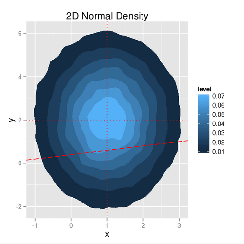
Let’s start by taking a look at the density of our 2D Gaussian:

n <- 100000
mu_x <- 1
mu_y <- 2
sigma_x <- 1
sigma_y <- 2

x <- rnorm(n, mean = mu_x, sd = sigma_x)
y <- rnorm(n, mean = mu_y, sd = sigma_y)

var_z <- sigma_x^2 + sigma_y^2

beta <- sigma_x^2 / var_z
alpha <- mu_x - beta * (mu_x + mu_y)

df <- data.frame(x, y)
ggplot(df, aes(x = x, y = y)) +
  stat_density2d(aes(fill = ..level..), geom="polygon") +
  geom_abline(intercept = alpha, slope = beta, color = "red",
  	linetype = "longdash") +
  geom_vline(xintercept = mu_x, color = "red", linetype = "dotted") +
  geom_hline(yintercept = mu_y, color = "red", linetype = "dotted") +
  theme(plot.background = element_rect(fill = '#F1F1F1'),
  	legend.background = element_rect(fill = '#F1F1F1')) +
	ggtitle("2D Normal Density")

The density above resulted from the sum of two independent normal distributions $N(1, 1)$ and $N(2, 2)$ . As such, it’s centered at $(1, 2)$ , and elongated along the $y$ axis. Plugging in the parameters of our distributions gives $\alpha = .4$ and $\beta = .2$ . Fitting the simulation data we find that our equation holds:

summary(lm(x ~ z))

Call:
lm(formula = x ~ z)

Residuals:
    Min      1Q  Median      3Q     Max
-3.5625 -0.6019 -0.0021  0.6016  3.9475

Coefficients:
            Estimate Std. Error t value Pr(>|t|)
(Intercept) 0.400942   0.004733   84.71   <2e-16 ***
z           0.199886   0.001263  158.29   <2e-16 ***
---
Signif. codes:  0 ‘***’ 0.001 ‘**’ 0.01 ‘*’ 0.05 ‘.’ 0.1 ‘ ’ 1

Residual standard error: 0.8946 on 99998 degrees of freedom
Multiple R-squared: 0.2004,	Adjusted R-squared: 0.2004
F-statistic: 2.506e+04 on 1 and 99998 DF,  p-value: < 2.2e-16

Note that $R^2 = .2$ , the same as our value of $\beta$ . For a simple linear regression $R^2$ is simply the squared correlation coefficient, or in our case:

\begin{aligned} R^2 &= \left(\frac{Cov(x, y)}{\sigma_x\sigma_y}\right)^2 \\ &= \frac{\sigma_x^2}{\sigma_x^2 + \sigma_y^2} = \beta \end{aligned}

That gives us a cool new interpretation of $\beta$ as the proportion of variance explained. It does however hint at a shortcoming that $R^2$ has as a goodness of fit measure—it explicitly depends on how our regressors are distributed.

At this point we have a simple formula to calculate a very useful conditional expectation. We also have a nice geometric interpretation of the solution, and an understanding that both regression and our original signal extraction problem distill down to a ratio of variances. Fantastic. However, we’re assuming that we know the proper, fixed parametrization of our model: $(\mu_1, \mu_2, \sigma_1, \sigma_2)$ , and that’s pretty unlikely. How do we estimate these parameters for a time-variant system given that we can only observe a series of $Z \sim z$ ? There are a myriad of approaches, each with pros, cons, and assumptions. Mixture models and machine learning are growing in favor for many applications. The CDS approach usually involves posing the model as a state space and estimating the parameters online. There’s no easy way out when faced with a partially observed, non-stationary process. So sorry folks—when it comes to denoising your signal, the equation above is the easy part.